Credit Score Classification: Leakage-Aware Evaluation & Risk-Averse Deployment

A leakage-aware machine learning pipeline for classifying customer credit scores using group-based validation, automated preprocessing, and conservative deployment logic.

Scikit-LearnXGBoostImbalanced-LearnStreamlitPython

Source Code Live Demo

Live Interactive Demo

Overview

This project classifies customer credit scores into three categories: Poor, Standard, and Good.

The dataset contains monthly financial records, meaning the same customer appears multiple times across different periods. This made the validation strategy just as important as the model itself. With a conventional random split, records from one customer could appear in both the training and test sets, allowing the model to learn customer-specific patterns instead of generalizing to unseen customers.

To prevent that issue, the project uses customer-aware data splitting, group-based cross-validation, reusable preprocessing, and an end-to-end deployment pipeline.

My Contribution

This was a group machine learning project. My main responsibilities were:

leading the technical design of the project,
preparing the data ingestion and initial preprocessing workflow,
designing the customer-aware validation strategy,
building the Logistic Regression baseline,
developing the CreditScoreDataWrangler custom transformer,
integrating the trained pipeline into a Streamlit application, and
implementing the Risk-Averse inference rule used during deployment.

The Random Forest and XGBoost experiments were developed collaboratively by other team members and evaluated through the same shared workflow.

The Main Challenge: Customer-Level Leakage

Each customer has several monthly observations. If those records are split randomly by row, the model may see one customer's earlier records during training and that same customer's later records during testing.

That produces an evaluation score that looks convincing but does not represent performance on genuinely unseen customers.

The initial holdout set was therefore created using GroupShuffleSplit, with Customer_ID used as the grouping key.

terminal

splitter = GroupShuffleSplit(
    n_splits=1,
    test_size=0.2,
    random_state=42
)

train_idx, test_idx = next(
    splitter.split(
        df,
        groups=df["Customer_ID"]
    )
)

train_df = df.iloc[train_idx].copy()
test_df = df.iloc[test_idx].copy()

This keeps every record belonging to one customer entirely within either the training or test set.

Hyperparameter tuning follows the same principle through five-fold StratifiedGroupKFold. It preserves customer boundaries while also maintaining a reasonably consistent target distribution across folds.

terminal

sgkf = StratifiedGroupKFold(
    n_splits=5,
    shuffle=True,
    random_state=42
)

This setup makes the final evaluation more representative of how the model would perform when receiving data from a new customer.

Data Preparation

The raw dataset required several cleaning steps before modeling.

Some numerical columns were stored as strings and contained invalid characters, while Credit_History_Age used values such as:

terminal

15 Years and 11 Months

These values were parsed into numeric month counts. Invalid values in fields such as age, interest rate, number of loans, bank accounts, and credit cards were converted into missing values before imputation.

Non-predictive identifiers were also removed:

terminal

columns_to_drop = [
    "ID",
    "SSN",
    "Name"
]

The remaining preprocessing logic was encapsulated in a reusable Scikit-Learn transformer named CreditScoreDataWrangler.

Custom Preprocessing Transformer

The CreditScoreDataWrangler handles the preprocessing operations that must remain consistent between training and inference.

Its main responsibilities include:

Customer-level imputation

Missing values are first forward-filled using earlier records from the same Customer_ID.
Training-based fallback values

Remaining numerical and categorical values are filled using medians and modes learned only from the training data.
Feature engineering

Payment_Behaviour is separated into spending and payment-value indicators, while Type_of_Loan is expanded into individual loan-type features.
Outlier capping

Numerical features are clipped using the 1st and 99th percentile boundaries learned during training.
Categorical encoding

Selected categorical features are converted into one-hot encoded columns.
Schema alignment

Data received during inference is reindexed to match the exact feature structure learned during training.

terminal

class CreditScoreDataWrangler(
    BaseEstimator,
    TransformerMixin
):
    def fit(self, X, y=None):
        X_fit = X.copy()

        columns = self.num_cols + self.cat_cols
        X_fit[columns] = (
            X_fit
            .groupby("Customer_ID")[columns]
            .ffill()
        )

        self.global_medians_ = (
            X_fit[self.num_cols]
            .median()
        )

        self.global_modes_ = (
            X_fit[self.cat_cols]
            .mode()
            .iloc[0]
        )

        X_fit = self._engineer_features(X_fit)

        for column in self.num_cols:
            self.capping_bounds_[column] = (
                X_fit[column].quantile(0.01),
                X_fit[column].quantile(0.99)
            )

        self.trained_columns_ = (
            self._prepare_model_features(X_fit)
            .columns
            .tolist()
        )

        return self

By storing the learned medians, modes, capping boundaries, and final feature schema, the transformer prevents the preprocessing logic used during deployment from drifting away from the training workflow.

Modeling Strategy

Three algorithms were evaluated:

Model	Role in the Experiment
Logistic Regression	Interpretable linear baseline
Random Forest	Non-linear ensemble using bagging
XGBoost	Gradient-boosted trees for more complex feature relationships

Because the target classes were imbalanced, model selection was not based on accuracy alone.

The class distribution was approximately:

Standard: 53%
Poor: 29%
Good: 18%

The primary optimization metric was therefore Macro F1, which gives equal importance to all three classes regardless of their frequency.

Macro Precision and Macro Recall were also included to evaluate whether a model performed consistently across the majority and minority classes.

Handling Class Imbalance

The XGBoost pipeline uses RandomOverSampler to increase the representation of minority classes during training.

The sampler is placed inside an ImbPipeline:

terminal

xgb_pipeline = ImbPipeline([
    (
        "wrangler",
        CreditScoreDataWrangler(
            num_cols=num_cols,
            cat_cols=cat_cols,
            drop_first=False,
            drop_vif_features=False
        )
    ),
    (
        "sampler",
        RandomOverSampler(
            random_state=42
        )
    ),
    (
        "classifier",
        XGBClassifier(
            objective="multi:softprob",
            eval_metric="mlogloss",
            random_state=42,
            tree_method="hist"
        )
    )
])

Because resampling occurs inside the pipeline, it is applied only to the training portion of each cross-validation fold. Validation records are never duplicated or included in the oversampling process.

This prevents resampled observations from leaking into model evaluation.

Hyperparameter Tuning

Each model was tuned using the same group-aware cross-validation strategy and optimized using Macro F1.

For XGBoost, the search covered:

number of estimators,
tree depth,
learning rate,
row subsampling,
column subsampling, and
minimum child weight.

terminal

xgb_param_dist = {
    "classifier__n_estimators": [
        200,
        400,
        600
    ],
    "classifier__max_depth": [
        4,
        6,
        8
    ],
    "classifier__learning_rate": [
        0.01,
        0.05,
        0.1
    ],
    "classifier__subsample": [
        0.8,
        1.0
    ],
    "classifier__colsample_bytree": [
        0.8,
        1.0
    ],
    "classifier__min_child_weight": [
        1,
        3,
        5
    ]
}

RandomizedSearchCV was used to evaluate parameter combinations without the computational cost of an exhaustive grid search.

Model Comparison

The tuned models were evaluated on a separate test set containing approximately 20,000 records.

Algorithm	Accuracy	Macro Precision	Macro Recall	Macro F1
Logistic Regression	0.61	0.61	0.67	0.61
Random Forest	0.69	0.67	0.73	0.68
XGBoost	0.70	0.68	0.73	0.69

XGBoost produced the strongest overall result, achieving the highest Accuracy, Macro Precision, and Macro F1.

Random Forest reached the same Macro Recall, but XGBoost provided a slightly better balance between precision and recall across the three classes.

The improvement over Logistic Regression also suggests that the relationship between the financial features and credit-score categories is not entirely linear.

Class-Level Performance

The overall metrics only show part of the result. Class-level evaluation provides a clearer view of the model's behavior.

The Logistic Regression baseline achieved a 0.83 recall for the Good class, but its recall for the Standard class fell to 0.48. This means the linear model detected many Good customers, but struggled to preserve the boundary of the majority class.

XGBoost produced a more balanced result:

0.81 recall for Good
0.76 recall for Poor
0.83 precision for Standard

The model gave up a small amount of Good-class recall compared with Logistic Regression, but performed more consistently across all three credit-score categories.

Confusion Matrix

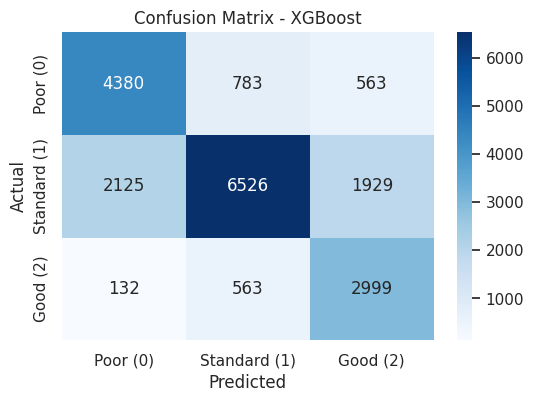
The confusion matrix shows that most remaining errors occur between neighboring risk categories.

One positive result is that only 132 customers who actually belonged to the Good class were classified as Poor. This indicates that the model rarely moved a low-risk customer directly into the highest-risk category.

The more important issue appeared in predictions assigned to the Good class:

1,929 Standard customers were predicted as Good
563 Poor customers were predicted as Good

These cases matter because incorrectly assigning a customer to the Good category is potentially riskier than making a conservative prediction.

That observation motivated the additional decision rule used in the deployed application.

Inspecting Feature Importance

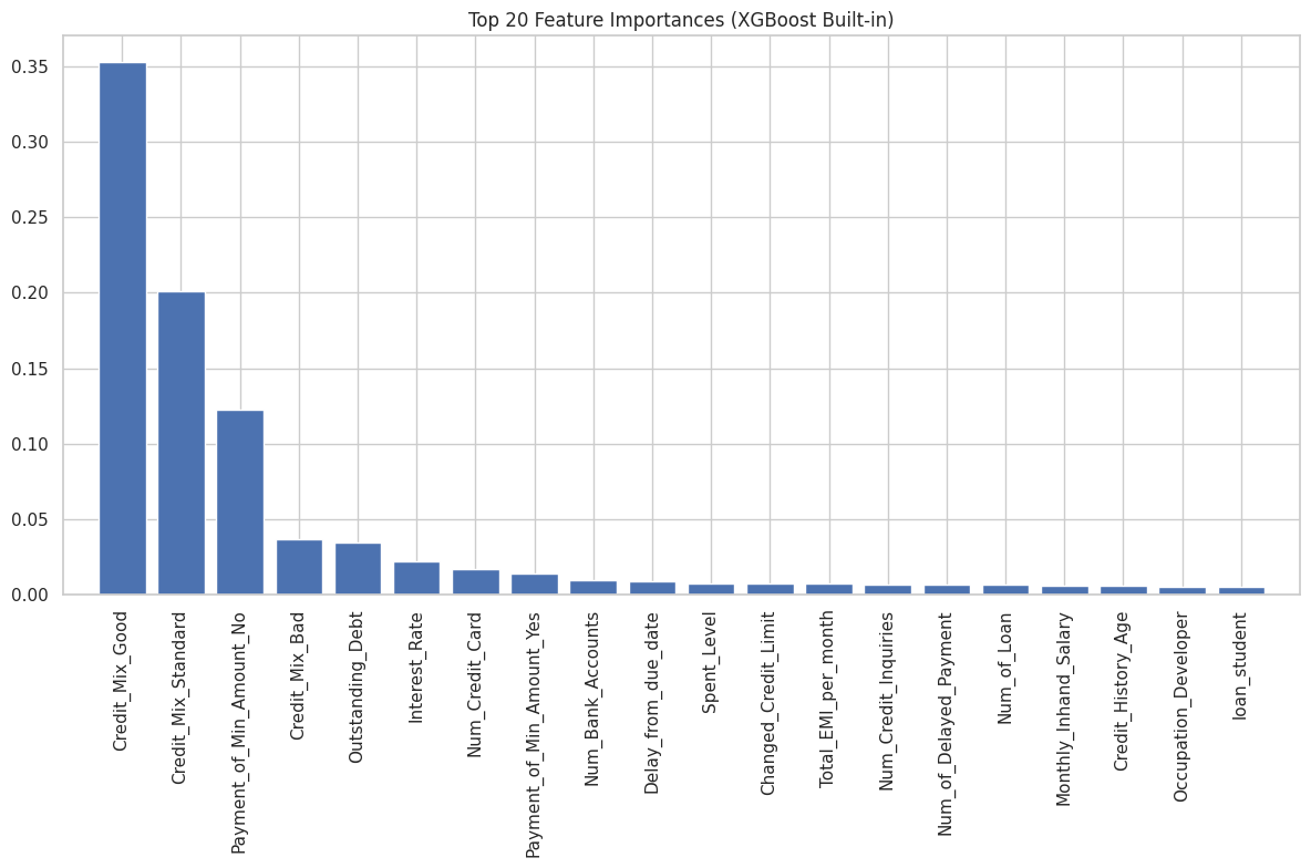
The built-in XGBoost feature importance indicates that the model relies heavily on features representing a customer's existing credit profile.

The three most influential features were:

Credit_Mix_Good
Credit_Mix_Standard
Payment_of_Min_Amount_No

Other relevant features included:

Credit_Mix_Bad
Outstanding_Debt
Interest_Rate
Num_Credit_Card
Payment_of_Min_Amount_Yes
Num_Bank_Accounts
Delay_from_due_date

This ranking shows which features contributed most frequently to the tree-building process.

It does not explain the direction of an individual prediction, but it provides a useful global view of the variables the model relied on most during training.

Deployment

The final XGBoost pipeline was exported as a serialized artifact and integrated into a Streamlit application.

Because the artifact stores both the fitted CreditScoreDataWrangler and the trained XGBoost classifier, the application can reuse the medians, modes, percentile boundaries, encoded columns, and model parameters learned during training.

The application allows users to:

enter customer financial information,
generate a credit-score prediction,
inspect the probability assigned to each class, and
compare the model's raw prediction with the Risk-Averse result.

Risk-Averse Inference

Using the class with the highest probability is not always the most appropriate decision rule for a risk-sensitive application.

The confusion matrix showed that some Poor and Standard customers were still predicted as Good. To demonstrate a more conservative inference strategy, the Streamlit application applies a 35% Poor-class threshold.

When the predicted probability of the Poor class reaches or exceeds 35%, the final output is changed to Poor even when another class has the highest raw probability.

terminal

class_labels = [
    "Poor",
    "Standard",
    "Good"
]

raw_probabilities = (
    model
    .predict_proba(X_input)[0]
)

poor_threshold = 0.35

if raw_probabilities[0] >= poor_threshold:
    final_prediction = "Poor"
else:
    final_prediction = class_labels[
        np.argmax(raw_probabilities)
    ]

For example, a raw probability distribution of:

terminal

Poor:     36%
Standard: 39%
Good:     25%

would normally produce a Standard prediction through argmax.

With the conservative override, the final result becomes Poor because the estimated Poor-class risk exceeds the configured threshold.

This rule is part of the deployment demonstration rather than the training process. It shows how model probabilities can be combined with an application-level policy when different prediction errors carry different consequences.

What I Learned

The most important lesson from this project was that a reliable evaluation design can matter more than selecting a more complex algorithm.

A model evaluated with customer leakage may produce impressive metrics without demonstrating genuine generalization. Keeping each customer isolated across the training, validation, and test partitions created a more realistic estimate of model performance.

The project also reinforced several practical lessons:

preprocessing should store its learned parameters for later inference,
resampling should happen only inside the training portion of cross-validation,
imbalanced multiclass problems should not be evaluated using accuracy alone,
class-level errors can reveal risks hidden by aggregate metrics, and
deployment decisions may require additional rules beyond the model's raw argmax output.

Final Result

The final system combines:

customer-aware train-test splitting,
five-fold StratifiedGroupKFold,
reusable preprocessing through a custom transformer,
oversampling inside an ImbPipeline,
XGBoost hyperparameter tuning,
multiclass evaluation using Macro F1, and
an interactive Streamlit deployment with conservative inference logic.

XGBoost achieved a 0.69 Macro F1, with 0.81 recall for Good customers and 0.76 recall for Poor customers.

More importantly, the project demonstrates an end-to-end workflow that considers not only predictive performance, but also data separation, reproducibility, class imbalance, error analysis, and deployment behavior.

A more detailed explanation of the methodology and experiments is available in the full report:

Read the Credit Score Classification Report

Arya's Portfolio

Credit Score Classification: Leakage-Aware Evaluation & Risk-Averse Deployment

Overview

My Contribution

The Main Challenge: Customer-Level Leakage

Data Preparation

Custom Preprocessing Transformer

Modeling Strategy

Handling Class Imbalance

Hyperparameter Tuning

Model Comparison

Class-Level Performance

Confusion Matrix

Inspecting Feature Importance

Deployment

Risk-Averse Inference

What I Learned

Final Result